What is the relationship between valve flow coefficients Cv and Kv?

Cv is expressed in US customary units (US GPM of 60°F water at 1 psi pressure drop), whereas Kv is expressed in SI metric units (m³/h of 15°C water at 1 bar pressure drop). The conversion factor is Cv = 1.156 * Kv (or Kv = 0.865 * Cv).

How do you determine if liquid flow through a valve is subcritical or critical?

Compare the actual pressure drop across the valve (ΔP) against the critical pressure drop limit ΔP_max = F_L^2 * ΔP_s. If ΔP = F_L^2 * ΔP_s, flow is critical (choked or flashing/cavitation occurs), and flow capacity no longer increases with further downstream pressure reduction.

What rule of thumb should be used for control valve pressure drop sizing?

A standard rule of thumb is that the control valve dynamic pressure drop should account for roughly 33% (1/3) of the total dynamic head loss of the piping system at normal flow rate, and the valve should operate between 20% and 80% open.

Valves Cv and Kv

Control valves Cv Kv flow coefficients for valve sizing

Volumetric and mass flow of liquid and gas through valves of coefficients Cv

Follow us on Twitter
Question, remark ? Contact us at contact@myengineeringtools.com

Quick Jump Table of Contents:

Cv and Kv definition
⚡ Interactive Cv / Kv Valve Flow Sizing Calculator
Calculation of Cv and flow - Case of liquids (SI units)
Calculation of Cv and flow - Case of gases (SI units)
Control valves sizing best practices
Corrections of Cv for special cases (Reducers & Viscosity)
Calculation of flow through a valve (US units)

1. Cv and Kv definition

What is the flow coefficient Cv and Kv - calculation of flow through a valve - SI units

The flow through a valve can be calculated thanks to the pressure drop through the valve and a coefficient Kv which represents the number of m³/h of water that goes through the valve at 15°C and with a pressure drop of 1 bar.

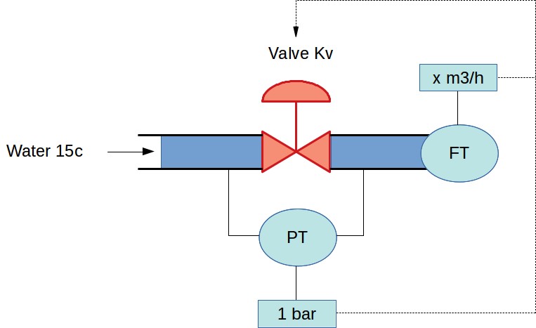
Manufacturers may specify the coefficient Cv instead of Kv for their valve. Cv is the number of US gallons that goes through the valve at 60°F and with a pressure drop of 1 psi. It is actually possible to convert Kv and Cv and have the expression in the right unit for the calculation of interest.

$ C_v = 1.156 \cdot K_v \quad \Longleftrightarrow \quad K_v = 0.865 \cdot C_v $

⚡ Interactive Control Valve Cv / Flow Calculator

Units: SI Metric US Imperial

⚠️ ENGINEERING NOTICE & EDUCATIONAL DISCLAIMER: This interactive calculator is provided exclusively for preliminary estimation and educational purposes. It is not intended for detailed design or equipment procurement without certified vendor rating. No warranty, expressed or implied, is provided, and no liability is assumed.

Calculation Target:

Fluid Type:

Valve Cv Coefficient (GPM):

Volumetric Flow Qv (m³/h):

Upstream Pressure P₁ (bar abs):

Pressure Drop ΔP (bar):

Liquid Density ρ (kg/m³) / SG:

Vapor Pressure Pv (bar abs):

Critical Pressure Pc (bar abs):

Recovery Factor FL:

Flow Regime: -

Calculated Valve Cv (GPM): -

Calculated Valve Kv (m³/h): -

Volumetric Flow Qv: -

Choked / Max Pressure Drop Limit: -

2. Calculation of Cv and flow through a valve - Case of liquids - SI units

What is the flow of liquid through a valve ?

2.1 Subcritical or critical flow ?

In order to calculate the flow of liquid through a valve thanks to the Cv, the Engineer must 1^st determine if the flow is subcritical or critical (cavitation / flashing). To do so, it is necessary to compare the pressure drop to some limit values.

If $\Delta P < F_L^2 (\Delta P_s)$ : the flow is subcritical
If $\Delta P \ge F_L^2 (\Delta P_s)$ : the flow is critical

With:

$\Delta P$ = Pressure drop across the valve (bar abs)
$F_L$ = liquid pressure recovery factor = $\sqrt{\frac{P_1 - P_2}{P_1 - P_{VC}}}$
$P_1$ = upstream pressure (bar abs)
$P_2$ = downstream pressure (bar abs)
$P_{VC}$ = pressure at the vena contracta of the valve (bar abs)
$\Delta P_s$ = critical pressure drop = $P_1 - \left(0.96 - 0.28 \cdot \sqrt{P_v / P_c}\right) \cdot P_v$
$P_v$ = vapor pressure of the liquid at the flow temperature (bar abs)
$P_c$ = pressure at thermodynamic critical point (bar abs)

The liquid pressure recovery factor is given by the valve manufacturer
$\Delta P_s$ can be approximated as $\Delta P_s = P_1 - P_v$ if $P_v < 0.5 \cdot P_1$

The relations given below are valid only for a Newtonian liquid in turbulent flow.

2.2 Subcritical flow

The volumetric flow of liquid through a valve can be calculated by $Q_v = K_v \cdot \sqrt{\Delta P / d}$ or $Q_v = \frac{C_v}{1.156} \cdot \sqrt{\Delta P / d}$ for subcritical flow.

\[ C_v = 1.156 \cdot Q_v \cdot \sqrt{\frac{d_{15}^t}{\Delta P}} \]

\[ Q_v = \frac{C_v}{1.156} \cdot \sqrt{\frac{\Delta P}{d_{15}^t}} \]

\[ Q_v = K_v \cdot \sqrt{\frac{\Delta P}{d_{15}^t}} \]

With:

$Q_v$ = Flow rate (m³/h)
$C_v$ = valve flow coefficient (GPM)
$K_v$ = valve flow coefficient (m³/h)
$\Delta P$ = Pressure drop across the valve (bar)
$d_{15}^t$ = density of the liquid referred to water at 15°C (-) - as density of water at this temperature is 999.13 kg/m³, $d_{15}^t$ can be approximated as $\rho / 1000$
$\rho$ = density of the liquid at flow temperature (kg/m³)

The mass flow rate through the valve can be calculated thanks to the formula $C_v = \frac{1.156 \cdot \dot{m}}{\sqrt{d_{15}^t \times \Delta P}} \implies \dot{m} = \frac{C_v}{1.156} \cdot \sqrt{d_{15}^t \times \Delta P}$:

\[ C_v = \frac{1.156 \cdot \dot{m}}{\sqrt{d_{15}^t \times \Delta P}} \quad \implies \quad \dot{m} = \frac{C_v}{1.156} \cdot \sqrt{d_{15}^t \times \Delta P} \]

With $\dot{m}$ = Flow rate (t/h).

2.3 Critical flow

For critical flow, the following formula can be used to calculate the volumetric flow through a valve of coefficient Cv:

\[ C_v = \frac{1.156 \cdot Q_v}{F_L} \cdot \sqrt{\frac{d_{15}^t}{\Delta P_s}} \quad \implies \quad Q_v = \frac{F_L \cdot C_v}{1.156} \cdot \sqrt{\frac{\Delta P_s}{d_{15}^t}} \]

For calculating the mass flow in critical flow:

\[ C_v = \frac{1.156 \cdot \dot{m}}{F_L \cdot \sqrt{d_{15}^t \times \Delta P_s}} \quad \implies \quad \dot{m} = \frac{F_L \cdot C_v \cdot \sqrt{d_{15}^t \times \Delta P_s}}{1.156} \]

Calculation example of the flow through a valve of coefficient Cv

A control valve has a Cv of 5. The instrumentation on the line shows that the pressure drop through the valve is 0.5 bar. What is the flow through the valve? It is water at 50°C.

The density of water at 15°C is 999.13 kg/m³.

The density of water at 50°C is 988.07 kg/m³.

The specific gravity of water at 50°C compared to water at 15°C is: 988.07 / 999.13 = 0.9889.

The flowrate is $Q_v = \frac{C_v}{1.156} \cdot \sqrt{\Delta P / d} = \frac{5}{1.156} \cdot \sqrt{0.5 / 0.9889} = 3.07 \text{ m}^3\text{/h}$.

3. Calculation of Cv and flow through a valve - Case of gases - SI units

What is the flow of gases through a valve ?

The volumetric flow rate of gas through a valve can be calculated from the valve Cv thanks to the following formula:

\[ C_v = \frac{Q_v \cdot \sqrt{d \cdot T \cdot Z}}{257 \cdot F_L \cdot P_1 \cdot \left(y - 0.148 \cdot y^3\right)} \quad \implies \quad Q_v = \frac{257 \cdot F_L \cdot C_v \cdot P_1 \cdot \left(y - 0.148 \cdot y^3\right)}{\sqrt{d \cdot T \cdot Z}} \]

With:

$Q_v$ = Flow rate (m³/h) at 15°C and 101,325 Pa abs
$F_L$ = critical flow factor
$C_v$ = valve flow coefficient (GPM)
$P_1$ = upstream pressure (bar abs)
$d$ = gas specific gravity vs air ($d_{\text{air}} = 1$) = $M / 28.96$
$M$ = molar mass of the gas (g/mol)
$T$ = temperature (K)
$Z$ = compressibility factor (-)
$y = \frac{1.63}{F_L} \cdot \sqrt{\frac{\Delta P}{P_1}}$

If $y < 1.5$, subcritical flow
If $y \ge 1.5$, critical flow and $y$ is capped at $y_{\text{max}} = 1.5$

The mass flowrate through the valve can be calculated thanks to the following formula:

\[ C_v = \frac{54.5 \cdot \dot{m} \cdot \sqrt{Z}}{F_L \cdot P_1 \cdot \sqrt{\frac{d \times 288}{T}} \cdot \left(y - 0.148 \cdot y^3\right)} \quad \implies \quad \dot{m} = \frac{F_L \cdot C_v \cdot P_1 \cdot \sqrt{\frac{d \times 288}{T}} \cdot \left(y - 0.148 \cdot y^3\right)}{54.5 \cdot \sqrt{Z}} \]

With $\dot{m}$ = Flow rate (t/h).

4. Control valve sizing best practices & Rules of Thumb

💡 Industrial Process Engineering Rules of Thumb

Pressure Drop Share: In standard pump/piping loop design, allocate 33% (1/3) of total dynamic system friction loss to the control valve (minimum 0.7 bar / 10 psi) to ensure sufficient authority over process flow.
Operating Opening Range: Size the valve so that normal flow rate occurs at 50% to 70% open, maximum design flow at <80% to 85% open, and minimum flow at >20% open.
Overdesign Margin: Apply a 10% to 20% margin on calculated flow rate before selecting the final catalog valve $C_v$ to account for pump wear and operating transients.
Avoid Cavitation: Ensure liquid $\Delta P < F_L^2 (P_1 - F_F P_v)$. If cavitation is unavoidable, specify hardened trim (Stellite/tungsten carbide) or anti-cavitation multi-stage trims.
Pipe Velocity Limits: Control valve inlet pipe velocity should remain below 3.0 m/s (10 ft/s) for liquids and 0.3 Mach for compressible gases to prevent excessive acoustic noise and erosion.

5. Corrections of Cv for special cases

5.1 Effect of pipe reducers

The formulas given above are valid when the valve diameter is equal to the pipe diameter. However, it sometimes happens that the valve is mounted in between pipe reducers, which reduces the effective capacity of the valve. To account for this effect, a coefficient $F_p$, the piping geometry factor, is calculated. The actual required Cv is then:

$ C_{v,\text{corrected}} = \frac{C_v}{F_p} $

\[ F_p = \left( \frac{C_v^2 \cdot \sum K}{0.00214 \cdot d^4} + 1 \right)^{-1/2} \]

With:

$C_{v,\text{corrected}}$ = actual Cv of the valve between pipe reducers
$C_v$ = calculated Cv without pipe reducers
$F_p$ = pipe geometry factor
$d$ = valve diameter (mm)
$\sum K = K_1 + K_2 + K_{B1} - K_{B2}$
$K_1$ = loss coefficient at inlet = $0.5 \cdot \left[1 - (d / D_1)^2\right]^2$
$K_2$ = loss coefficient at outlet = $\left[1 - (d / D_2)^2\right]^2$
$K_{B1}$ = Bernoulli coefficient = $1 - (d / D_1)^4$
$K_{B2}$ = Bernoulli coefficient = $1 - (d / D_2)^4$
$D_1$ = inside diameter of upstream pipe (mm)
$D_2$ = inside diameter of downstream pipe (mm)

5.2 Effect of viscosity

According to [Baumann], the correction of the valve Cv due to viscosity is to be applied only if the fluid has a kinematic viscosity > 40 centistokes. The correction procedure requires the calculation of a correction factor $F_R$ which will be used in a similar way as the coefficient $F_p$ for pipe geometry.

5.3 Laminar flow

The case of laminar flow is according to Baumann calculated the same way as a correction of viscosity, which appears logical as a higher viscosity will often lead to laminar flow.

6. Calculation of flow through a valve - US units

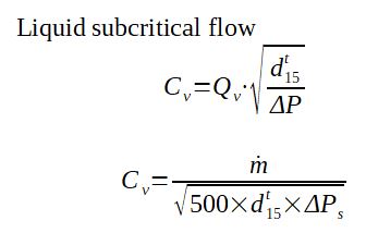
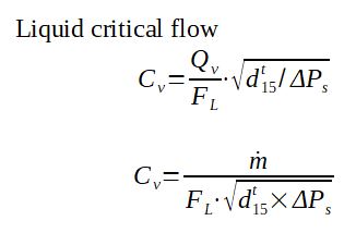
The relations above, in US customary units, are expressed in the following ways to calculate valves of Cv in liquid and gas applications:

Liquid Subcritical Flow (US Units):

\[ C_v = Q_v \cdot \sqrt{\frac{d_{15}^t}{\Delta P}} \quad ; \quad C_v = \frac{\dot{m}}{\sqrt{500 \times d_{15}^t \times \Delta P_s}} \]

CV valve calculation US units liquid subcritical flow

Liquid Critical Flow (US Units):

\[ C_v = \frac{Q_v}{F_L} \cdot \sqrt{\frac{d_{15}^t}{\Delta P_s}} \quad ; \quad C_v = \frac{\dot{m}}{F_L \cdot \sqrt{d_{15}^t \times \Delta P_s}} \]

CV valve calculation US units liquid critical flow

Gas Flow (US Units):

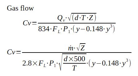
\[ C_v = \frac{Q_v \cdot \sqrt{d \cdot T \cdot Z}}{834 \cdot F_L \cdot P_1 \cdot \left(y - 0.148 \cdot y^3\right)} \quad ; \quad C_v = \frac{\dot{m} \cdot \sqrt{Z}}{2.8 \times F_L \cdot P_1 \cdot \sqrt{\frac{d \times 500}{T}} \cdot \left(y - 0.148 \cdot y^3\right)} \]

With $P$ and $\Delta P$ in psi abs / psi, $Q_v$ in US GPM (liquids) or SCFH (gas), $C_v$ in GPM, $\dot{m}$ in lb/h, $d$ is specific gravity (water = 1 at 60°F), $T$ flowing temperature in °R.

Source:

Masoneilan Control Valve Sizing Handbook, 2000